Multi-Asset Momentum Strategy in R

Click and see the complete code

1) Determine 8 indexes which is representing each asset
2) Get Long Momentum (105 days) and Short Momentum (20 days) to rank
3) Determine the category with the lowest sum of the two ranks. (1st + 5th = 6)
4) To see if the current price is higher than the past 3-month average.
    If it is higher, then do invest


required(quantmod, PerformanceAnalytics, TTR)


#get adjust prices

symbols <- c("NAESX", #small cap "PREMX", #emerging bond "VEIEX", #emerging markets "VFICX", #intermediate investment grade "VFIIX", #GNMA mortgage "VFINX", #S&P 500 index "VGSIX", #MSCI REIT "VGTSX", #total intl stock idx "VUSTX") #long term treasury (cash)

getSymbols(symbols, from="1990-01-01")


#save to Prices

prices <- list() for(i in 1:length(symbols)) { prices[[i]] <- Ad(get(symbols[i])[,6]) }

#change to Dataframe and remove NA values

prices <- cbind="" colnames="" do.call="" gsub="" na.omit="" prices="" span="" z="">

#split cash apart from ranking calculation

cashPrices<-prices font="" prices="">

#calculate momentum

nShort <- 20="" span="">

nLong <- 105="" span="">

nSMA <- 3="" span="">

momShort <- -="" 1="" lag="" nshort="" prices="" span="">

momLong <- -="" 1="" lag="" nlong="" prices="" span="">

PricesQ<-prices endpoints="" on="quarters" prices="" span="">

PricesM<-prices endpoints="" on="months" prices="" span="">

momShortQ<-momshort endpoints="" on="quarters" prices="" span="">

momLongQ<-momlong endpoints="" on="quarters" prices="" span="">

#rank by momentum

srank <- 1="" apply="" br="" lrank="" momlongq="" momshortq="" rank="" t="">

#as there is a chance that both values are same, I put more value on long momentum totRank <- 1.01="" 1="" apply="" function="" lrank="" max="" maxrank="" rankpos="" rankrow="" return="" span="" srank="" t="" totrank="">

# check whether current price is higher than average of past 3 months prices.

PricesSMAsM<- apply="" index="" n="nSMA)," order.by="index(PricesM))" pricesq="" pricessmasm="" pricessmasq="" ricesm="" ricesq="" smafilter="" xts=""> PricesSMAsQ

[출처] 해외주식 투자하기 7편. 멀티에셋 모멘텀 전략|작성자 엉드루

# find intersections between the two

lastPos<- br="" lastpos="" na.omit="" rankpos="" smafilter="">

#invest to cash if there is nothing to invest cash <- cash="" font="" join="inner" lastpos="" merge="" order.by="index(lastPos))" rowsums="" xts="">

#calculate return

prices<-merge cashprices="" eturn.calculate="" font="" join="inner" lastpos="" na.omit="" prices="" return.portfolio="" returns="" stratrets="">

#evaluate the model

table.AnnualizedReturns(stratRets) maxDrawdown(stratRets) charts.PerformanceSummary(stratRets)

portfolio.returns Annualized Return 0.1680 Annualized Std Dev 0.1599 Annualized Sharpe (Rf=0%) 1.0507

maxDrawndown=[1] 0.2978453

-reference-

http://blog.naver.com/htk1019/220924952051

[출처] 해외주식 투자하기 7편. 멀티에셋 모멘텀 전략|작성자 엉드루

[출처] 해외주식 투자하기 7편. 멀티에셋 모멘텀 전략|작성자 엉드루

Financial Data Web Scraping/Parsing Sample in Python

Financial data scraping from finviz.
http://finviz.com/


required : beautifulsoup and pandas

How to collect financial data in R

Click and see complete code

Two jobs we have to do.

1) to get a specific company financial data
2) to show several companies' financial ratio

--------------------------------------------------------------

Let's start do the first job.

#basic setting and get an object
     library(quantmod)
     nvdia=getFinancials("NVDA", auto.assign = FALSE)

#Annual and Quarter Balance sheet

     nvdia.BS.A=viewFinancials(nvdia, type='BS', period='A')

     nvdia.BS.Q=viewFinancials(nvdia, type='BS', period='Q')

#Income Statement

     nvdia.IS.A = viewFinancials(nvdia, type='IS', period='A')

     nvdia.IS.Q = viewFinancials(nvdia, type='IS', period='Q')

#cash flow

     nvdia.CF.A = viewFinancials(nvdia, type='CF', period='A')

     nvdia.CF.Q = viewFinancials(nvdia, type='CF', period='Q')

#check netincome

      rownames(nvdia.IS.A)

 [1] "Revenue"                                         

 [2] "Other Revenue, Total"                            

 [3] "Total Revenue"                                   

 [4] "Cost of Revenue, Total"                          

 [5] "Gross Profit"           

                        

------

[25] "Net Income"              

-------

                              

[48] "Basic Normalized EPS"                            

[49] "Diluted Normalized EPS" 

Now, number 25 abbreviates netincome

nvdia.IS.A[25,]

2017-01-29 2016-01-31 2015-01-25 2014-01-26 

   1666.00     614.00     630.59     439.99 

------------------------------------------------------------------------------

2) Let's show several companies' financial status using yahooQF

#make a list you want to find out

Ratios <- ales="" c="" div="" nbsp="" rice="" yahooqf="">

                    "P/E Ratio", 

                    "Price/EPS Estimate Next Year", 

                    "PEG Ratio", 

                    "Dividend Yield", 

                    "Market Capitalization"))

#make a list of companies you want to look at

codes <- c="" div="">

#combine and get rid of date

FinancialRatio<- codes="" collapse=";" getquote="" paste="" sep="" what="Ratios)</div">

FinancialRatio <- data.frame="" div="" financialratio="" inancialratio="" length="" ymbol="codes,">

FinancialRatio

     Symbol Price.Sales P.E.Ratio

GOOG   GOOG        6.57     30.31

IBM     IBM        1.90     13.06

MSFT   MSFT        6.06     30.64

ORCL   ORCL        4.94     21.31

NVDA   NVDA        8.89     41.49

AAPL   AAPL        3.46     17.60

     Price.EPS.Estimate.Next.Year PEG.Ratio

GOOG                        23.29      1.38

IBM                         11.39      4.57

MSFT                        21.16      2.41

ORCL                        15.92      1.95

NVDA                        31.55      3.14

AAPL                        14.26      1.74

     Dividend.Yield Market.Capitalization

GOOG            N/A               627.25B

IBM            3.74               149.23B

MSFT           2.28               536.05B

ORCL           1.42               185.37B

NVDA           0.54                62.81B

AAPL           1.59               769.04B

That's all

-reference-

http://blog.naver.com/htk1019/220913777513

Basic System Trading Based on Machine Learning (SVM)

click for complete code

snp<- span="" style="color: #9cdcfe;">getSymbols

('^GSPC', src='yahoo', auto.assign = FALSE)

ret<- span="" style="color: #9cdcfe;">snp

[,4]-snp[,1])/snp[,1]

ret = ret['2007-01-01/2017-04-28']

y=ret

y[y>0.000]=1

y[y<=0.000]=0

x = Lag(y, k=1)

for(i in 2:5)

{

x = cbind(x,Lag(y,k=i))

}

data = cbind(y, x,ret)

data<- span="" style="color: #dcdcaa;">na.omit

(data))

inputs <- span="" style="color: #9cdcfe;">data

[,2:5]

outputs <- span="" style="color: #9cdcfe;">data

[,c(1,7)]

datacnt = length(outputs[,1])

outsvm = c()

n_train = 30

for(i in n_train : (datacnt-1))

{

train = c((i-n_train+1):i)

fitsvm<- span="" style="color: #9cdcfe;">svm

(inputs[train,],outputs[train,1], kernel='linear')

predsvm <- span="" style="color: #dcdcaa;">predict

(fitsvm, inputs[i+1,])

actual <- span="" style="color: #9cdcfe;">outputs

[i+1,2]

outsvm = rbind(outsvm, c(date=rownames(as.data.frame(inputs)[i+1,]),pred=predsvm,act=actual))

print(paste(sep="", as.character((i-n_train+1)/(datacnt-n_train-1)*100),"% done"))

}

simData=as.matrix(outsvm,ncol=3)

simData[,2][as.double(simData[,2])>=0.5]=1

simData[,2][as.double(simData[,2])<0.5]=0

simData[,3] = as.double(simData[,3])

ret = as.numeric(simData[,2])*as.numeric(simData[,3])

ret = as.data.frame(ret)

rownames(ret) = simData[,1]

portCumRet = exp(cumsum(ret))

chartSeries(portCumRet)

simData=as.matrix(outsvm,ncol=3)

simData[,2][as.double(simData[,2])<0.5]=-1

simData[,2][as.double(simData[,2])>=0.5]=0

simData[,3] = as.double(simData[,3])

ret = as.numeric(simData[,2])*as.numeric(simData[,3])

ret = as.data.frame(ret)

rownames(ret) = simData[,1]

portCumRet = exp(cumsum(ret))

chartSeries(portCumRet)

A graph of the second strategy looks really horrible.

Wish you guys have a beautiful one.

Sorted

-reference-

http://blog.naver.com/htk1019/220911828081

[출처] 해외주식 투자하기 4편. R을 활용한 기술적 분석 2탄 - 머신러닝을 이용한 나만의 기술적 지표|작성자 엉드루

[출처] 해외주식 투자하기 4편. R을 활용한 기술적 분석 2탄 - 머신러닝을 이용한 나만의 기술적 지표|작성자 엉드루

[출처] 해외주식 투자하기 4편. R을 활용한 기술적 분석 2탄 - 머신러닝을 이용한 나만의 기술적 지표|작성자 엉드루

[출처] 해외주식 투자하기 4편. R을 활용한 기술적 분석 2탄 - 머신러닝을 이용한 나만의 기술적 지표|작성자 엉드루

[출처] 해외주식 투자하기 4편. R을 활용한 기술적 분석 2탄 - 머신러닝을 이용한 나만의 기술적 지표|작성자 엉드루

[출처] 해외f주식 투자하기 ㅈ4편. R을 활용한 기술적 분석 2탄 - 머신러닝을 이용한 나만의 기술적 지표|작성자 엉드루

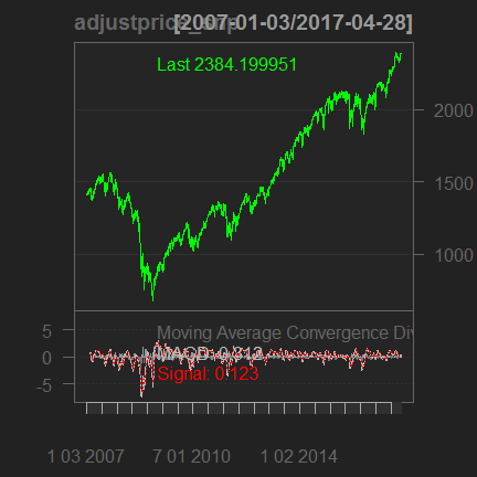
Technical Analysis in R (addMACD)

*Due to html problem, some codes are broken,
 so download a complete code in my google drive please
Click and download the code


required packages : quantmod / PerformanceAnalytics


1) collect data, S&P 500 index
      snp <- auto.assign="FALSE)</p" getsymbols="" src="yahoo">
2) take only adjust price
      adjustprice_snp<-snp -snp="" p="">
3) Draw MACD chart
      chartSeries(adjustprice_snp, TA="addMACD()")

4) adjust variable in macd analysis
      macd =

 MACD(adjustprice_snp, nFast=15, nSlow=30,nSig=9,maType=SMA, percent = FALSE)


5) create trading signal
    signal = Lag(ifelse(macd$macd>=macd$signal, 1,0))

-get rid of lookahead bias by lagging
-trade based on signal

6) calculate return
     ret = ROC(adjustprice_snp)*signal

7) set time
    ret = ret['2009-01-01/2017-01-10']

8) calculate cumulative return
    portCumRet = exp(cumsum(ret))
    plot(portCumRet)

9) evaluate risk
   #check worst 10 period and downside risk
     table.Drawdowns(ret,top=10)
     table.DownsideRisk(ret)     

     charts.PerformanceSummary(ret)

#other functions for technical analysis including MACD
addADX
add Welles Wilder's Directional Movement Indicator*
addATR
add Average True Range *
addBBands:
add Bollinger Bands *
addCCI
add Commodity Channel Index *
addCMF
add Chaiken Money Flow *
addCMO
add Chande Momentum Oscillator *
addDEMA
add Double Exponential Moving Average *
addDPO
add Detrended Price Oscillator *
addEMA
add Exponential Moving Average *
addEnvelope
add Moving Average Envelope
addEVWMA
add Exponential Volume Weighted Moving Average *
addExpiry
add options or futures expiration lines
addLines
add line(s)
addMACD:
add Moving Average Convergence Divergence *
addMomentum
add Momentum *
addPoints
add point(s) 
addROC:
add Rate of Change *
addRSI
add Relative Strength Indicator *
addSAR
add Parabolic SAR *
addSMA
add Simple Moving Average *
addSMI
add Stochastic Momentum Index *
addTRIX
add Triple Smoothed Exponential Oscillator *
addVo:
add Volume if available
addWMA
add Weighted Moving Average *
addWPR
add Williams Percent R *
addZLEMA


-reference-
http://blog.naver.com/htk1019/220908871667

[출처] 해외주식 투자하기 4편. R을 활용한 기술적 분석|작성자 엉드루

[출처] 해외주식 투자하기 4편. R을 활용한 기술적 분석|작성자 엉드루

How to collect price in R

I'd like to show you how to use R to get global stock prices.

it is freaking easy.

just enter following code to get S&P 500 index.


getSymbols('^GSPC', src='yahoo')
plot(GSPC)

It's too easy, isnt it?

If you trying to find out Nvida's stock price, then enter NVDA instead of ^GSPC.


nvda <- auto.assign="FALSE)</p" getsymbols="" src="yahoo">plot(nvda)

Sorted

*Additional information

Free financial data

1) R package quantmod

:yahoo(stock information) / google(stock data)

:FRED(economic indicators)

:Oanda(FX data)

example) Oanda

getSymbols("USD/EUR",src="oanda")

plot(USDEUR)

2) R package Quandl (not all free but some of them are free)

example) Quandl

Let's get oil price and draw a graph

install.packages("Quandl")
library(Quandl)data = Quandl("OPEC/ORB")

3) R package TFX which provides real time tick data

Sample)

install.packages("TFX")
QueryTrueFX()
yen <- span=""> ConnectTrueFX("USD/JPY,EUR/JPY,GBP/JPY,AUD/JPY,CAD/JPY,CHF/JPY", 
                     username="ID", password="PW")
QueryTrueFX(yen)

4) R package pwt which provides global economic data

Sample)

install.packages("pwt8")

library("pwt8") 

data("pwt8.0")

countries <- c="" div="">

variables <- c="" country="" div="" isocode="" nbsp="" pop="" rgdpo="" year="">

pwt <- countries="" in="" isocode="" pwt8.0="" select="variables)</div" subset="">

summary(pwt)

                     country      isocode  

 Spain                   :62   ESP    :62  

 Italy                   :62   ITA    :62  

 United States of America:62   USA    :62  

 Angola                  : 0   AGO    : 0  

 Albania                 : 0   ALB    : 0  

 Argentina               : 0   ARG    : 0  

 (Other)                 : 0   (Other): 0  

      year          rgdpo         

 Min.   :1950   Min.   :   85002  

 1st Qu.:1965   1st Qu.:  439149  

 Median :1980   Median : 1107030  

 Mean   :1980   Mean   : 2722070  

 3rd Qu.:1996   3rd Qu.: 3536036  

 Max.   :2011   Max.   :13193478

5) R package - rdatamarket



-reference-
http://blog.naver.com/htk1019/220902013375

[출처] 해외주식 투자하기 1-1편. 무료 금융 데이터소스 정리|작성자 엉드루

[출처] 해외주식 투자하기 1-1편. 무료 금융 데이터소스 정리|작성자 엉드루

How to collect economic data from FRED in R

How to collect economic data from FRED

At least you should have a basic understanding of analytical tools, R and Python.

Also, it is assumed that R and quantmod(package) have been already installed.

First of all, Have a look at a indicator you want to find
1) if you succeed to access the website, FRED, you can see the following screen.
2)  just type US Recession Probabilities






There are two search results,
of which Smoothed U.S Recession Probabilities is the economic index I want.

Do you see the code RECPROUSM156N next to the indicator name?
Please keep it in mind.

Next stage is to download the data from R

And we are going to use getSymbols in guantmod.

codes are following:

install.packages("quantmod")
library(quantmod)
getSymbols("RECPROUSM156N", src='FRED')
plot(RECPROUSM156N)

Tada~Here we are, that's it.

A variation of the code is to use several index at the same time.
Let's find out relation between Kospi index and the recession probabilities.


require(quantmod)

rec<-getsymbols auto.assign="FALSE)<br" src="FRED">kospi<-getsymbols auto.assign="FALSE)</span" src="yahoo">


# to data.frame
dfrec <- as.data.frame="" br="" rec="">dfkospi <- as.data.frame="" kospi="" lose="" span="">
mrec<- cbind="" eval_d="row.names(dfrec)," rec="dfrec)<br">mkospi<- cbind="" eval_d="row.names(dfkospi)," kospi="dfkospi)</span">
merged_rec_kospi<-merge br="" by="eval_d" mkospi="" mrec="">plot(merged_rec_kospi[,2], type='l', col='red')
par(new=TRUE)
plot(merged_rec_kospi[,3], type='l', col='blue')




it can be found that when the recession probabilities increased rapidly,
there is a high chance that the kospi index would slumped.

-reference-
http://blog.naver.com/htk1019/220891514114

How to read thesis/papers efficiently ? - 논문을 효과적으로 읽는 방법

How to read papers effectively:

When you reading a thesis, it is effective to read it three times in different ways.

1. firstly, understand approximate ideas

2. Reading the papers for a second time: understand rest of contents

3. Reading the papers for a third time: understanding the thesis deeply

First pass:

Within 5-10 minutes

- Read title, abstract and introduction

- Read only list of contents, understand a structure of the paper and skip the rest of them boldly

- Read the conclusion

- Understand purpose of the paper while roughly reading the reference

After the first pass, you should be able to answer the following questions:

1. Category: What type of paper is this?

2. Context: What other papers are related? Which theories were used to analyze the problem?

3. Correctness: Are the assumptions valid?

4. Contributions: What are papers' main contributions?

5. Clarity: Is the paper well written?

Second pass:

- within a hour

- Read carefully, but skip such a detail like a process of proof

- Write a list of important questions in the margin and write down questions you would like to ask the author.

- Look at graphs, figures

Third pass:

- More than 2 hours

- Restructure a paper with an idea that I would write my paper again in my head

- Make sure you understand the assumptions between all sentences and make sure that the assumptions are correct.

- Think about how you would present the ideas in this article

- Write new ideas in the margin

- After reading, remember the whole structure of this paper.

------------------------------------------------------------------------------------------------------------------------------

논문을 효과적으로 읽는법:

논문을 읽을때 총 세번 다른 방법으로 읽는게 효과적임
1. 첫번째로 읽을때: 대략적인 아이디어 파악
2. 두번째로 읽을때: 디테일을 제외한 내용 파악
3. 세번째로 읽을때: 논문을 깊이 이해

First pass:
- 5-10 분 이내
- 제목, abstract, intro 를 읽음
- section 과 subsection 제목만 읽고 나머지는 과감히 스킵
- 결론을 읽음
- reference를 대충 읽으면서 이미 읽은 논문이 어떤건지 대충 파악

First pass가 끝나면 아래의 질문들에 대해서 답할 수 있어야 함
1. Category: what type of paper is this?
2. Context: What other papers are related? Which theories were used to analyze the problem?
3. Correctness: Are the assumptions valid?
4. Contributions: What are papers’ main contributions?
5. Clarity: Is the paper well written?

Second pass:
- 한 시간 이내
- 좀 더 자세히 읽되 증명 같이 너무 detail 한 것들 스킵
- 중요 내용들을 여백에 정리하면서 저자에게 물어보고 싶은 질문들도 적어놓음
- graphs, figure들을 눈여겨 볼것

Third pass:
- 2시간 이상
- 아예 논문을 머릿속에서 다시 써본다는 생각을 가지고 읽음
- 모든 문장 뒤에 있는 assumption을 확실히 이해하고, 그 assumption이 맞는지 확인해볼것
- 과연 나 같으면 어떤식으로 이 논문에 있는 아이디어를 제시할지 생각해볼것
- 새로운 아이디어들을 여백에 적음
- 읽고 나면 이 논문의 전체 구조를 기억할 수 있어야함

-reference-

Owen Song