Showing posts with label R. Show all posts

02/05/2017

How to calculate correlation coefficients for US stock sectors

Click and see the complete code


#required

library(dplyr)
library(quantmod)
library(dygraphs)


#get etf data from http://www.sectorspdr.com/sectorspdr/ 

tickers<- c="" p="">sectorNames <- c="" discretionary="" nbsp="" onsumer="" p="" staples="">                 "Energy", "Financials", "Health Care", "Industrials",
                 "Materials", "Information Technology", "Utilities", "Index")
etf_ticker_sectors <- data_frame="" p="" sectornames="" tickers="">
#check data
etf_ticker_sectors

# # A tibble: 10 × 2
# tickers            sectorNames
#                  
#   1      XLY Consumer Discretionary
# 2      XLP       Consumer Staples
# 3      XLE                 Energy
# 4      XLF             Financials
# 5      XLV            Health Care
# 6      XLI            Industrials
# 7      XLB              Materials
# 8      XLK Information Technology
# 9      XLU              Utilities
# 10     SPY                  Index


#calculate weekly return

sector_weekly_returns <- function="" p="" tickers="">
#download data
  symbols <- auto.assign="TRUE," getsymbols="" tickers="" warnings="FALSE)</p">
#get only close price
  prices <- cl="" do.call="" function="" get="" lapply="" merge="" p="" symbols="" x="">
#calculate weekly log-based return using a function, periodReturn()
  weekly_returns <- do.call="" lapply="" merge="" nbsp="" p="" prices="">                                          function(x) periodReturn(x, period = 'weekly', type = 'log')))


#Change the column names to the sector names from our dataframe above.

  colnames(weekly_returns) <- div="" etf_ticker_sectors="" sectornames="">
  return(weekly_returns)

}

weekly_returns = sector_weekly_returns(tickers)

weekly_returns
# 2008-10-10 -0.2205639196
# 2008-10-17  0.0518524493
# 2008-10-24 -0.0684872067
# 2008-10-31  0.1065890897
# 2008-11-07 -0.0311525633
# 2008-11-14 -0.0802735506
# 2008-11-21 -0.0855222458
# 2008-11-28  0.1248006016


#get rolling correlation between sector etf and s&p 500 etf

sector_index_correlation <- function="" p="" window="" x="">
#merge return of sector  and s&p500
  merged_xts <- merge="" ndex="" p="" weekly_returns="" x="">
#calculate rolling correlations using rollapply()
#pairwise.complete.obs automatically removes NA

  merged_xts$rolling_cor <- merged_xts="" nbsp="" p="" rollapply="" window="">                                      function(x) cor(x[,1], x[,2], use = "pairwise.complete.obs"),
                                      by.column = FALSE)

  names(merged_xts) <- c="" correlation="" ector="" p="" returns="">
  return(merged_xts)
}

#use a created function we made above

IT_SPY_correlation <- p="" sector_index_correlation="">  weekly_returns$'Information Technology', 26)

#draw graph using Dygragh

dygraph(IT_SPY_correlation$'Sector/SPY Correlation', main = "Correlation between SP500 and Tech ETF") %>%
  dyAxis("y", label = "Correlation") %>%
  dyRangeSelector(height = 20) %>%
  # Add shading for the recessionary period
  dyShading(from = "2007-12-01", to = "2009-06-01", color = "#FFE6E6") %>%
  # Add an event for the financial crisis.
  dyEvent(x = "2008-09-15", label = "Fin Crisis", labelLoc = "top", color = "red")


-reference-
http://blog.naver.com/htk1019/220966797230

How to calculate F-score in R

Click and see the complete code


#Get NVDA financial data for recent 3 years

library(quantmod)
NVDA    = getFinancials("NVDA",auto.assign = FALSE)
NVDA.BS = viewFinancials(NVDA, type='BS', period='A')
NVDA.IS = viewFinancials(NVDA, type='IS', period='A')
NVDA.CF = viewFinancials(NVDA, type='CF', period='A')


#Get the financial data to calculate F-Score

TA = NVDA.BS[rownames(NVDA.BS)=="Total Assets",]
CA = NVDA.BS[rownames(NVDA.BS)=="Total Current Assets",]
CL = NVDA.BS[rownames(NVDA.BS)=="Total Current Liabilities",]
NCL = NVDA.BS[rownames(NVDA.BS)=="Total Long Term Debt",]
NI = NVDA.IS[rownames(NVDA.IS)=="Net Income",]
CFO = NVDA.CF[rownames(NVDA.CF)=="Cash from Operating Activities",]
SALES = NVDA.IS[rownames(NVDA.IS)=="Revenue",]
NUMSHARES = NVDA.BS[rownames(NVDA.BS)=="Total Common Shares Outstanding",]
GP = NVDA.IS[rownames(NVDA.IS)=="Gross Profit",]


#calculate financial ratio

ROA = NI/TA
TURN = SALES/TA
CR = CA/CL
LDE = NCL / TA
GM = GP/SALES

#conditions for fscore

F1 = as.integer(ROA[1]>0)
F2 = as.integer(CFO[1]>0)
F3 = as.integer((CFO-NI)[1]>0)
F4 = as.integer(NUMSHARES[1]-NUMSHARES[2]<=0)
F5 = as.integer(TURN[1]-TURN[2]>0)
F6 = as.integer(CR[1]-CR[2]>0)
F7 = as.integer(LDE[1]-LDE[2]<=0)
F8 = as.integer(GM[1]-GM[2]>0)
F9 = as.integer(ROA[1]-ROA[2]>0)

F = F1+F2+F3+F4+F5+F6+F7+F8+F9


#define function

getFScore <-function code="" p="">{

  Company    = getFinancials(code,auto.assign = FALSE)
  Company.BS = viewFinancials(Company, type='BS', period='A')
  Company.IS = viewFinancials(Company, type='IS', period='A')
  Company.CF = viewFinancials(Company, type='CF', period='A')

  TA = Company.BS[rownames(Company.BS)=="Total Assets",]
  CA = Company.BS[rownames(Company.BS)=="Total Current Assets",]
  CL = Company.BS[rownames(Company.BS)=="Total Current Liabilities",]
  NCL = Company.BS[rownames(Company.BS)=="Total Long Term Debt",]
  NI = Company.IS[rownames(Company.IS)=="Net Income",]
  CFO = Company.CF[rownames(Company.CF)=="Cash from Operating Activities",]
  SALES = Company.IS[rownames(Company.IS)=="Revenue",]
  NUMSHARES = Company.BS[rownames(Company.BS)=="Total Common Shares Outstanding",]
  GP = Company.IS[rownames(Company.IS)=="Gross Profit",]

  ROA = NI/TA
  TURN = SALES/TA
  CR = CA/CL
  LDE = NCL / TA
  GM = GP/SALES

  F1 = as.integer(ROA[1]>0)
  F2 = as.integer(CFO[1]>0)
  F3 = as.integer((CFO-NI)[1]>0)
  F4 = as.integer(NUMSHARES[1]-NUMSHARES[2]<=0)
  F5 = as.integer(TURN[1]-TURN[2]>0)
  F6 = as.integer(CR[1]-CR[2]>0)
  F7 = as.integer(LDE[1]-LDE[2]<=0)
  F8 = as.integer(GM[1]-GM[2]>0)
  F9 = as.integer(ROA[1]-ROA[2]>0)

  F_SCORE = F1+F2+F3+F4+F5+F6+F7+F8+F9

  return (F_SCORE)
}

codes <- c="" p="">CompanyFscores = c()
for(code in codes)
{
  CompanyFscores=rbind(CompanyFscores,getFScore(code))
}
rownames(CompanyFscores) = codes
colnames(CompanyFscores) = "FScore"

CompanyFscores

#result
     FScore
GOOG      6
IBM       5
MSFT      5
ORCL      5
NVDA      7
AAPL      5


-reference-
http://blog.naver.com/htk1019/220955604506

Multi-Asset Momentum Strategy in R


Click and see the complete code

1) Determine 8 indexes which is representing each asset
2) Get Long Momentum (105 days) and Short Momentum (20 days) to rank
3) Determine the category with the lowest sum of the two ranks. (1st + 5th = 6)
4) To see if the current price is higher than the past 3-month average.
    If it is higher, then do invest


required(quantmod, PerformanceAnalytics, TTR)


#get adjust prices

symbols <- c("NAESX", #small cap "PREMX", #emerging bond "VEIEX", #emerging markets "VFICX", #intermediate investment grade "VFIIX", #GNMA mortgage "VFINX", #S&P 500 index "VGSIX", #MSCI REIT "VGTSX", #total intl stock idx "VUSTX") #long term treasury (cash)

getSymbols(symbols, from="1990-01-01")


#save to Prices

prices <- list() for(i in 1:length(symbols)) { prices[[i]] <- Ad(get(symbols[i])[,6]) }


#change to Dataframe and remove NA values

prices <- cbind="" colnames="" do.call="" gsub="" na.omit="" prices="" span="" z="">


#split cash apart from ranking calculation

cashPrices<-prices font="" prices="">


#calculate momentum


nShort <- 20="" span="">
nLong <- 105="" span="">
nSMA <- 3="" span="">

momShort <- -="" 1="" lag="" nshort="" prices="" span="">

momLong <- -="" 1="" lag="" nlong="" prices="" span="">

PricesQ<-prices endpoints="" on="quarters" prices="" span="">
PricesM<-prices endpoints="" on="months" prices="" span="">

momShortQ<-momshort endpoints="" on="quarters" prices="" span="">
momLongQ<-momlong endpoints="" on="quarters" prices="" span="">


#rank by momentum

srank <- 1="" apply="" br="" lrank="" momlongq="" momshortq="" rank="" t="">
#as there is a chance that both values are same, I put more value on long momentum totRank <- 1.01="" 1="" apply="" function="" lrank="" max="" maxrank="" rankpos="" rankrow="" return="" span="" srank="" t="" totrank="">


# check whether current price is higher than average of past 3 months prices.

PricesSMAsM<- apply="" index="" n="nSMA)," order.by="index(PricesM))" pricesq="" pricessmasm="" pricessmasq="" ricesm="" ricesq="" smafilter="" xts=""> PricesSMAsQ


# find intersections between the two

lastPos<- br="" lastpos="" na.omit="" rankpos="" smafilter="">
#invest to cash if there is nothing to invest cash <- cash="" font="" join="inner" lastpos="" merge="" order.by="index(lastPos))" rowsums="" xts="">


#calculate return

prices<-merge cashprices="" eturn.calculate="" font="" join="inner" lastpos="" na.omit="" prices="" return.portfolio="" returns="" stratrets="">


#evaluate the model

table.AnnualizedReturns(stratRets) maxDrawdown(stratRets) charts.PerformanceSummary(stratRets)

portfolio.returns Annualized Return 0.1680 Annualized Std Dev 0.1599 Annualized Sharpe (Rf=0%) 1.0507
maxDrawndown=[1] 0.2978453


-reference-
http://blog.naver.com/htk1019/220924952051


How to collect financial data in R

Click and see complete code

Two jobs we have to do.

1) to get a specific company financial data
2) to show several companies' financial ratio

--------------------------------------------------------------

Let's start do the first job.

#basic setting and get an object
     library(quantmod)
     nvdia=getFinancials("NVDA", auto.assign = FALSE)

#Annual and Quarter Balance sheet
     nvdia.BS.A=viewFinancials(nvdia, type='BS', period='A')
     nvdia.BS.Q=viewFinancials(nvdia, type='BS', period='Q')

#Income Statement
     nvdia.IS.A = viewFinancials(nvdia, type='IS', period='A')
     nvdia.IS.Q = viewFinancials(nvdia, type='IS', period='Q')

#cash flow
     nvdia.CF.A = viewFinancials(nvdia, type='CF', period='A')
     nvdia.CF.Q = viewFinancials(nvdia, type='CF', period='Q')


#check netincome

      rownames(nvdia.IS.A)

 [1] "Revenue"                                         
 [2] "Other Revenue, Total"                            
 [3] "Total Revenue"                                   
 [4] "Cost of Revenue, Total"                          
 [5] "Gross Profit"           
                        
------
[25] "Net Income"              
-------
                              
[48] "Basic Normalized EPS"                            
[49] "Diluted Normalized EPS" 


Now, number 25 abbreviates netincome

nvdia.IS.A[25,]

2017-01-29 2016-01-31 2015-01-25 2014-01-26 
   1666.00     614.00     630.59     439.99 

------------------------------------------------------------------------------

2) Let's show several companies' financial status using yahooQF


#make a list you want to find out
Ratios <- ales="" c="" div="" nbsp="" rice="" yahooqf="">
                    "P/E Ratio", 
                    "Price/EPS Estimate Next Year", 
                    "PEG Ratio", 
                    "Dividend Yield", 
                    "Market Capitalization"))


#make a list of companies you want to look at
codes <- c="" div="">

#combine and get rid of date
FinancialRatio<- codes="" collapse=";" getquote="" paste="" sep="" what="Ratios)</div">

FinancialRatio <- data.frame="" div="" financialratio="" inancialratio="" length="" ymbol="codes,">

FinancialRatio


     Symbol Price.Sales P.E.Ratio
GOOG   GOOG        6.57     30.31
IBM     IBM        1.90     13.06
MSFT   MSFT        6.06     30.64
ORCL   ORCL        4.94     21.31
NVDA   NVDA        8.89     41.49
AAPL   AAPL        3.46     17.60
     Price.EPS.Estimate.Next.Year PEG.Ratio
GOOG                        23.29      1.38
IBM                         11.39      4.57
MSFT                        21.16      2.41
ORCL                        15.92      1.95
NVDA                        31.55      3.14
AAPL                        14.26      1.74
     Dividend.Yield Market.Capitalization
GOOG            N/A               627.25B
IBM            3.74               149.23B
MSFT           2.28               536.05B
ORCL           1.42               185.37B
NVDA           0.54                62.81B
AAPL           1.59               769.04B


That's all

-reference-
http://blog.naver.com/htk1019/220913777513


01/05/2017

Basic System Trading Based on Machine Learning (SVM)

click for complete code


snp<- span="" style="color: #9cdcfe;">getSymbols
('^GSPC', src='yahoo', auto.assign = FALSE)

ret<- span="" style="color: #9cdcfe;">snp
[,4]-snp[,1])/snp[,1]
ret = ret['2007-01-01/2017-04-28']


y=ret
y[y>0.000]=1
y[y<=0.000]=0

x = Lag(y, k=1)
for(i in 2:5)
{
x = cbind(x,Lag(y,k=i))
}

data = cbind(y, x,ret)
data<- span="" style="color: #dcdcaa;">na.omit
(data))

inputs <- span="" style="color: #9cdcfe;">data
[,2:5]
outputs <- span="" style="color: #9cdcfe;">data
[,c(1,7)]

datacnt = length(outputs[,1])


outsvm = c()


n_train = 30

for(i in n_train : (datacnt-1))
{
train = c((i-n_train+1):i)

fitsvm<- span="" style="color: #9cdcfe;">svm
(inputs[train,],outputs[train,1], kernel='linear')
predsvm <- span="" style="color: #dcdcaa;">predict
(fitsvm, inputs[i+1,])
actual <- span="" style="color: #9cdcfe;">outputs
[i+1,2]
outsvm = rbind(outsvm, c(date=rownames(as.data.frame(inputs)[i+1,]),pred=predsvm,act=actual))
print(paste(sep="", as.character((i-n_train+1)/(datacnt-n_train-1)*100),"% done"))
}

simData=as.matrix(outsvm,ncol=3)

simData[,2][as.double(simData[,2])>=0.5]=1
simData[,2][as.double(simData[,2])<0.5]=0
simData[,3] = as.double(simData[,3])


ret = as.numeric(simData[,2])*as.numeric(simData[,3])
ret = as.data.frame(ret)
rownames(ret) = simData[,1]

portCumRet = exp(cumsum(ret))
chartSeries(portCumRet)


simData=as.matrix(outsvm,ncol=3)

simData[,2][as.double(simData[,2])<0.5]=-1
simData[,2][as.double(simData[,2])>=0.5]=0
simData[,3] = as.double(simData[,3])

ret = as.numeric(simData[,2])*as.numeric(simData[,3])
ret = as.data.frame(ret)
rownames(ret) = simData[,1]

portCumRet = exp(cumsum(ret))
chartSeries(portCumRet)


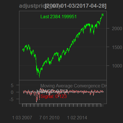
Technical Analysis in R (addMACD)

*Due to html problem, some codes are broken,
 so download a complete code in my google drive please
Click and download the code


required packages : quantmod / PerformanceAnalytics


1) collect data, S&P 500 index
      snp <- auto.assign="FALSE)</p" getsymbols="" src="yahoo">
2) take only adjust price
      adjustprice_snp<-snp -snp="" p="">
3) Draw MACD chart
      chartSeries(adjustprice_snp, TA="addMACD()")


4) adjust variable in macd analysis
      macd =
 MACD(adjustprice_snp, nFast=15, nSlow=30,nSig=9,maType=SMA, percent = FALSE)


5) create trading signal
    signal = Lag(ifelse(macd$macd>=macd$signal, 1,0))

-get rid of lookahead bias by lagging
-trade based on signal

6) calculate return
     ret = ROC(adjustprice_snp)*signal

7) set time
    ret = ret['2009-01-01/2017-01-10']

8) calculate cumulative return
    portCumRet = exp(cumsum(ret))
    plot(portCumRet)

9) evaluate risk
   #check worst 10 period and downside risk
     table.Drawdowns(ret,top=10)
     table.DownsideRisk(ret)
     
     charts.PerformanceSummary(ret)


#other functions for technical analysis including MACD
addADX
add Welles Wilder's Directional Movement Indicator*
addATR
add Average True Range *
addBBands:
add Bollinger Bands *
addCCI
add Commodity Channel Index *
addCMF
add Chaiken Money Flow *
addCMO
add Chande Momentum Oscillator *
addDEMA
add Double Exponential Moving Average *
addDPO
add Detrended Price Oscillator *
addEMA
add Exponential Moving Average *
addEnvelope
add Moving Average Envelope
addEVWMA
add Exponential Volume Weighted Moving Average *
addExpiry
add options or futures expiration lines
addLines
add line(s)
addMACD:
add Moving Average Convergence Divergence *
addMomentum
add Momentum *
addPoints
add point(s) 
addROC:
add Rate of Change *
addRSI
add Relative Strength Indicator *
addSAR
add Parabolic SAR *
addSMA
add Simple Moving Average *
addSMI
add Stochastic Momentum Index *
addTRIX
add Triple Smoothed Exponential Oscillator *
addVo:
add Volume if available
addWMA
add Weighted Moving Average *
addWPR
add Williams Percent R *
addZLEMA


-reference-
http://blog.naver.com/htk1019/220908871667